Computer Vision
约 8852 个字 167 张图片 预计阅读时间 44 分钟 共被读过 次
This note is based on GitHub - DaizeDong/Stanford-CS231n-2021-and-2022: Notes and slides for Stanford CS231n 2021 & 2022 in English. I merged the contents together to get a better version. Assignments are not included. 斯坦福 cs231n 的课程笔记 ( 英文版本,不含实验代码 ),将 2021 与 2022 两年的课程进行了合并,分享以供交流。
And I will add some blogs, articles and other understanding.
| Topic | Chapter |
|---|---|
| Deep Learning Basics | 2 - 4 |
| Perceiving and Understanding the Visual World | 5 - 12 |
| Reconstructing and Interacting with the Visual World | 13 - 16 |
| Human-Centered Applications and Implications | 17 - 18 |
1 - Introduction
A brief history of computer vision & deep learning...
2 - Image Classification
Image Classification: A core task in Computer Vision. The main drive to the progress of CV.
Challenges: Viewpoint variation, background clutter, illumination, occlusion, deformation, intra-class variation...
K Nearest Neighbor
Hyperparameters: Distance metric (\(p\) norm), \(k\) number.
Choose hyperparameters using validation set.
Never use k-Nearest Neighbor with pixel distance.
Linear Classifier
Pass...
3 - Loss Functions and Optimization
Loss Functions
| Dataset | \(\big\{(x_i,y_i)\big\}_{i=1}^N\\\) |
|---|---|
| Loss Function | \(L=\frac{1}{N}\sum_{i=1}^NL_i\big(f(x_i,W),y_i\big)\\\) |
| Loss Function with Regularization | \(L=\frac{1}{N}\sum_{i=1}^NL_i\big(f(x_i,W),y_i\big)+\lambda R(W)\\\) |
Motivation: Want to interpret raw classifier scores as probabilities.
| Softmax Classifier | \(p_i=Softmax(y_i)=\frac{\exp(y_i)}{\sum_{j=1}^N\exp(y_j)}\\\) |
|---|---|
| Cross Entropy Loss | \(L_i=-y_i\log p_i\\\) |
| Cross Entropy Loss with Regularization | \(L=-\frac{1}{N}\sum_{i=1}^Ny_i\log p_i+\lambda R(W)\\\) |
Optimization
SGD with Momentum
Problems that SGD can't handle:
- Inequality of gradient in different directions.
- Local minima and saddle point (much more common in high dimension).
- Noise of gradient from mini-batch.
Momentum: Build up “velocity” \(v_t\) as a running mean of gradients.
| SGD | SGD + Momentum |
|---|---|
| \(x_{t+1}=x_t-\alpha\nabla f(x_t)\) | \(\begin{align}&v_{t+1}=\rho v_t+\nabla f(x_t)\\&x_{t+1}=x_t-\alpha v_{t+1}\end{align}\) |
| Naive gradient descent. | \(\rho\) gives "friction", typically \(\rho=0.9,0.99,0.999,...\) |
Nesterov Momentum: Use the derivative on point \(x_t+\rho v_t\) as gradient instead point \(x_t\).
| Momentum | Nesterov Momentum |
|---|---|
| \(\begin{align}&v_{t+1}=\rho v_t+\nabla f(x_t)\\&x_{t+1}=x_t-\alpha v_{t+1}\end{align}\) | \(\begin{align}&v_{t+1}=\rho v_t+\nabla f(x_t+\rho v_t)\\&x_{t+1}=x_t-\alpha v_{t+1}\end{align}\) |
| Use gradient at current point. | Look ahead for the gradient in velocity direction. |
AdaGrad and RMSProp
AdaGrad: Accumulate squared gradient, and gradually decrease the step size.
RMSProp: Accumulate squared gradient while decaying former ones, and gradually decrease the step size. ("Leaky AdaGrad")
| AdaGrad | RMSProp |
|---|---|
| \(\begin{align}\text{Initialize:}&\\&r:=0\\\text{Update:}&\\&r:=r+\Big[\nabla f(x_t)\Big]^2\\&x_{t+1}=x_t-\alpha\frac{\nabla f(x_t)}{\sqrt{r}}\end{align}\) | \(\begin{align}\text{Initialize:}&\\&r:=0\\\text{Update:}&\\&r:=\rho r+(1-\rho)\Big[\nabla f(x_t)\Big]^2\\&x_{t+1}=x_t-\alpha\frac{\nabla f(x_t)}{\sqrt{r}}\end{align}\) |
| Continually accumulate squared gradients. | \(\rho\) gives "decay rate", typically \(\rho=0.9,0.99,0.999,...\) |
Adam
Sort of like "RMSProp + Momentum".
| Adam (simple version) | Adam (full version) |
|---|---|
| \(\begin{align}\text{Initialize:}&\\&r_1:=0\\&r_2:=0\\\text{Update:}&\\&r_1:=\beta_1r_1+(1-\beta_1)\nabla f(x_t)\\&r_2:=\beta_2r_2+(1-\beta_2)\Big[\nabla f(x_t)\Big]^2\\&x_{t+1}=x_t-\alpha\frac{r_1}{\sqrt{r_2}}\end{align}\) | \(\begin{align}\text{Initialize:}\\&r_1:=0\\&r_2:=0\\\text{For }i\text{:}\\&r_1:=\beta_1r_1+(1-\beta_1)\nabla f(x_t)\\&r_2:=\beta_2r_2+(1-\beta_2)\Big[\nabla f(x_t)\Big]^2\\&r_1'=\frac{r_1}{1-\beta_1^i}\\&r_2'=\frac{r_2}{1-\beta_2^i}\\&x_{t+1}=x_t-\alpha\frac{r_1'}{\sqrt{r_2'}}\end{align}\) |
| Build up “velocity” for both gradient and squared gradient. | Correct the "bias" that \(r_1=r_2=0\) for the first few iterations. |
Overview
 |  |
|---|---|
Learning Rate Decay
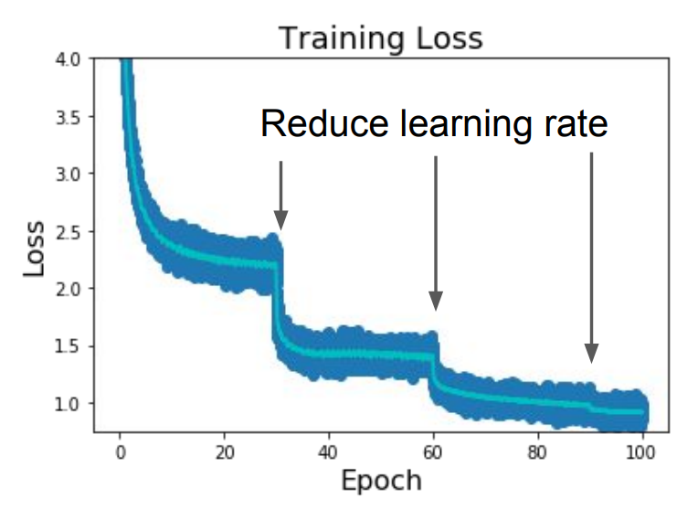
Reduce learning rate at a few fixed points to get a better convergence over time.
\(\alpha_0\) : Initial learning rate.
\(\alpha_t\) : Learning rate in epoch \(t\).
\(T\) : Total number of epochs.
High initial learning rates can make loss explode, linearly increasing learning rate in the first few iterations can prevent this.
Learning rate warm up:
Empirical rule of thumb: If you increase the batch size by \(N\), also scale the initial learning rate by \(N\) .
Second-Order Optimization
| Picture | Time Complexity | Space Complexity | |
|---|---|---|---|
| First Order |  | \(O(n)\) | \(O(n)\) |
| Second Order |  | \(O(n^2)\) with BGFS optimization | \(O(n)\) with L-BGFS optimization |
L-BGFS : Limited memory BGFS.
- Works very well in full batch, deterministic \(f(x)\).
- Does not transfer very well to mini-batch setting.
Summary
| Method | Performance |
|---|---|
| Adam | Often chosen as default method. Work ok even with constant learning rate. |
| SGD + Momentum | Can outperform Adam. Require more tuning of learning rate and schedule. |
| L-BGFS | If can afford to do full batch updates then try out. |
- An article about gradient descent: Anoverview of gradient descent optimization algorithms
- A blog: An updated overview of recent gradient descent algorithms – John Chen – ML at Rice University
4 - Neural Networks and Backpropagation
Neural Networks
Motivation: Inducted bias can appear to be high when using human-designed features.
Activation: Sigmoid, tanh, ReLU, LeakyReLU...
Architecture: Input layer, hidden layer, output layer.
Do not use the size of a neural network as the regularizer. Use regularization instead!
Gradient Calculation: Computational Graph + Backpropagation.
Backpropagation
Using Jacobian matrix to calculate the gradient of each node in a computation graph.
Suppose that we have a computation flow like this:
| Input X | Input W | Output Y |
|---|---|---|
| \(X=\begin{bmatrix}x_1\\x_2\\\vdots\\x_n\end{bmatrix}\) | \(W=\begin{bmatrix}w_{11}&w_{12}&\cdots&w_{1n}\\w_{21}&w_{22}&\cdots&w_{2n}\\\vdots&\vdots&\ddots&\vdots\\w_{m1}&w_{m2}&\cdots&w_{mn}\end{bmatrix}\) | \(Y=\begin{bmatrix}y_1\\y_2\\\vdots\\y_m\end{bmatrix}\) |
| \(n\times 1\) | \(m\times n\) | \(m\times 1\) |
After applying feed forward, we can calculate gradients like this:
| Derivative Matrix of X | Jacobian Matrix of X | Derivative Matrix of Y |
|---|---|---|
| \(D_X=\begin{bmatrix}\frac{\partial L}{\partial x_1}\\\frac{\partial L}{\partial x_2}\\\vdots\\\frac{\partial L}{\partial x_n}\end{bmatrix}\) | \(J_X=\begin{bmatrix}\frac{\partial y_1}{\partial x_1}&\frac{\partial y_1}{\partial x_2}&\cdots&\frac{\partial y_1}{\partial x_n}\\\frac{\partial y_2}{\partial x_1}&\frac{\partial y_2}{\partial x_2}&\cdots&\frac{\partial y_2}{\partial x_n}\\\vdots&\vdots&\ddots&\vdots\\\frac{\partial y_m}{\partial x_1}&\frac{\partial y_m}{\partial x_2}&\cdots&\frac{\partial y_m}{\partial x_n}\end{bmatrix}\) | \(D_Y=\begin{bmatrix}\frac{\partial L}{\partial y_1}\\\frac{\partial L}{\partial y_2}\\\vdots\\\frac{\partial L}{\partial y_m}\end{bmatrix}\) |
| \(n\times 1\) | \(m\times n\) | \(m\times 1\) |
| Derivative Matrix of W | Jacobian Matrix of W | Derivative Matrix of Y |
|---|---|---|
| \(W=\begin{bmatrix}\frac{\partial L}{\partial w_{11}}&\frac{\partial L}{\partial w_{12}}&\cdots&\frac{\partial L}{\partial w_{1n}}\\\frac{\partial L}{\partial w_{21}}&\frac{\partial L}{\partial w_{22}}&\cdots&\frac{\partial L}{\partial w_{2n}}\\\vdots&\vdots&\ddots&\vdots\\\frac{\partial L}{\partial w_{m1}}&\frac{\partial L}{\partial w_{m2}}&\cdots&\frac{\partial L}{\partial w_{mn}}\end{bmatrix}\) | \(J_W^{(k)}=\begin{bmatrix}\frac{\partial y_k}{\partial w_{11}}&\frac{\partial y_k}{\partial w_{12}}&\cdots&\frac{\partial y_k}{\partial w_{1n}}\\\frac{\partial y_k}{\partial w_{21}}&\frac{\partial y_k}{\partial w_{22}}&\cdots&\frac{\partial y_k}{\partial w_{2n}}\\\vdots&\vdots&\ddots&\vdots\\\frac{\partial y_k}{\partial w_{m1}}&\frac{\partial y_k}{\partial w_{m2}}&\cdots&\frac{\partial y_k}{\partial w_{mn}}\end{bmatrix}\) \(J_W=\begin{bmatrix}J_W^{(1)}&J_W^{(2)}&\cdots&J_W^{(m)}\end{bmatrix}\) | \(D_Y=\begin{bmatrix}\frac{\partial L}{\partial y_1}\\\frac{\partial L}{\partial y_2}\\\vdots\\\frac{\partial L}{\partial y_m}\end{bmatrix}\) |
| \(m\times n\) | \(m\times m\times n\) | $ m\times 1$ |
For each element in \(D_X\) , we have:
\(D_{Xi}=\frac{\partial L}{\partial x_i}=\sum_{j=1}^m\frac{\partial L}{\partial y_j}\frac{\partial y_j}{\partial x_i}\\\)
5 - Convolutional Neural Networks
Convolution Layer
Introduction
Convolve a filter with an image: Slide the filter spatially within the image, computing dot products in each region.
Giving a \(32\times32\times3\) image and a \(5\times5\times3\) filter, a convolution looks like:
Convolve six \(5\times5\times3\) filters to a \(32\times32\times3\) image with step size \(1\), we can get a \(28\times28\times6\) feature:
With an activation function after each convolution layer, we can build the ConvNet with a sequence of convolution layers:
By changing the step size between each move for filters, or adding zero-padding around the image, we can modify the size of the output:
\(1\times1\) Convolution Layer
This kind of layer makes perfect sense. It is usually used to change the dimension (channel) of features.
A \(1\times1\) convolution layer can also be treated as a full-connected linear layer.
Summary
| Input | |
|---|---|
| image size | \(W_1\times H_1\times C\) |
| filter size | \(F\times F\times C\) |
| filter number | \(K\) |
| stride | \(S\) |
| zero padding | \(P\) |
| Output | |
| output size | \(W_2\times H_2\times K\) |
| output width | \(W_2=\frac{W_1-F+2P}{S}+1\\\) |
| output height | \(H_2=\frac{H_1-F+2P}{S}+1\\\) |
| Parameters | |
| parameter number (weight) | \(F^2CK\) |
| parameter number (bias) | \(K\) |
Pooling layer
Make the representations smaller and more manageable.
An example of max pooling:
| Input | |
|---|---|
| image size | \(W_1\times H_1\times C\) |
| spatial extent | \(F\times F\) |
| stride | \(S\) |
| Output | |
| output size | \(W_2\times H_2\times C\) |
| output width | \(W_2=\frac{W_1-F}{S}+1\\\) |
| output height | \(H_2=\frac{H_1-F}{S}+1\\\) |
Convolutional Neural Networks (CNN)
CNN stack CONV, POOL, FC layers.
CNN Trends:
- Smaller filters and deeper architectures.
- Getting rid of POOL/FC layers (just CONV).
Historically architectures of CNN looked like:
where usually \(m\) is large, \(0\le n\le5\), \(0\le k\le2\).
Recent advances such as ResNet / GoogLeNet have challenged this paradigm.
6 - CNN Architectures
Best model in ImageNet competition:
AlexNet
8 layers.
First use of ConvNet in image classification problem.
Filter size decreases in deeper layer.
Channel number increases in deeper layer.
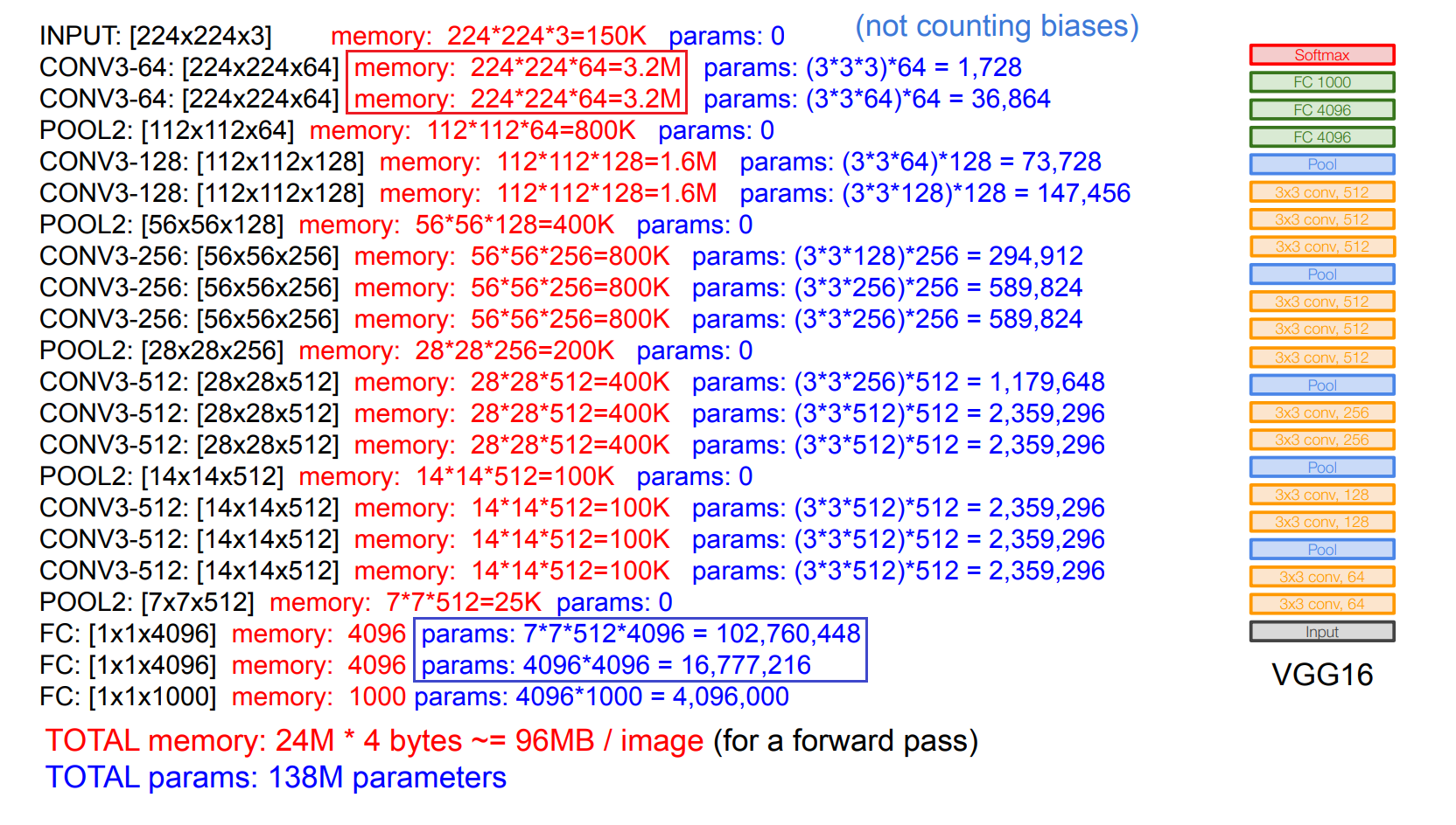
VGG
19 layers. (also provide 16 layers edition)
Static filter size (\(3\times3\)) in all layers:
- The effective receptive field expands with the layer gets deeper.
- Deeper architecture gets more non-linearities and few parameters.
Most memory is in early convolution layers.
Most parameter is in late FC layers.
GoogLeNet
22 layers.
No FC layers, only 5M parameters. ( \(8.3\%\) of AlexNet, \(3.7\%\) of VGG )
Devise efficient "inception module".
Inception Module
Design a good local network topology (network within a network) and then stack these modules on top of each other.
Naive Inception Module:
- Apply parallel filter operations on the input from previous layer.
- Concatenate all filter outputs together channel-wise.
- Problem: The depth (channel number) increases too fast, costing expensive computation.
Inception Module with Dimension Reduction:
- Add "bottle neck" layers to reduce the dimension.
- Also get fewer computation cost.
Architecture
ResNet
152 layers for ImageNet.
Devise "residual connections".
Use BN in place of dropout.
Residual Connections
Hypothesis: Deeper models have more representation power than shallow ones. But they are harder to optimize.
Solution: Use network layers to fit a residual mapping instead of directly trying to fit a desired underlying mapping.
It is necessary to use ReLU as activation function, in order to apply identity mapping when \(F(x)=0\) .
Architecture
SENet
Using ResNeXt-152 as a base architecture.
Add a “feature recalibration” module. (adjust weights of each channel)
Using the global avg-pooling layer + FC layers to determine feature map weights.
Improvements of ResNet
Wide Residual Networks, ResNeXt, DenseNet, MobileNets...
Other Interesting Networks
NASNet: Neural Architecture Search with Reinforcement Learning.
EfficientNet: Smart Compound Scaling.
7 - Training Neural Networks
Activation Functions
| Activation | Usage |
|---|---|
| Sigmoid, tanh | Do not use. |
| ReLU | Use as default. |
| Leaky ReLU, Maxout, ELU, SELU | Replace ReLU to squeeze out some marginal gains. |
| Swish | No clear usage. |
Data Processing
Apply centralization and normalization before training.
In practice for pictures, usually we apply channel-wise centralization only.
Weight Initialization
Assume that we have 6 layers in a network.
\(D_i\) : input size of layer \(i\)
\(W_i\) : weights in layer \(i\)
\(X_i\) : output after activation of layer \(i\), we have \(X_i=g(Z_i)=g(W_iX_{i-1}+B_i)\)
We initialize each parameter in \(W_i\) randomly in \([-k_i,k_i]\) .
| Tanh Activation | Output Distribution |
|---|---|
| \(k_i=0.01\) |  |
| \(k_i=0.05\) |  |
| Xavier Initialization \(k_i=\frac{1}{\sqrt{D_i}\\}\) |  |
When \(k_i=0.01\), the variance keeps decreasing as the layer gets deeper. As a result, the output of each neuron in deep layer will all be 0. The partial derivative \(\frac{\partial Z_i}{\partial W_i}=X_{i-1}=0\\\). (no gradient)
When \(k_i=0.05\), most neurons is saturated. The partial derivative \(\frac{\partial X_i}{\partial Z_i}=g'(Z_i)=0\\\). (no gradient)
To solve this problem, We need to keep the variance same in each layer.
Assuming that \(Var\big(X_{i-1}^{(1)}\big)=Var\big(X_{i-1}^{(2)}\big)=\dots=Var\big(X_{i-1}^{(D_i)}\big)\)
We have \(Z_i=X_{i-1}^{(1)}W_i^{(:,1)}+X_{i-1}^{(2)}W_i^{(:,2)}+\dots+X_{i-1}^{(D_i)}W_i^{(:,D_i)}=\sum_{n=1}^{D_i}X_{i-1}^{(n)}W_i^{(:,n)}\\\)
We want \(Var\big(Z_i\big)=Var\big(X_{i-1}^{(n)}\big)\)
Let's do some conduction:
\(\begin{aligned}Var\big(Z_i\big)&=Var\Bigg(\sum_{n=1}^{D_i}X_{i-1}^{(n)}W_i^{(:,n)}\Bigg)\\&=D_i\ Var\Big(X_{i-1}^{(n)}W_i^{(:,n)}\Big)\\&=D_i\ Var\Big(X_{i-1}^{(n)}\Big)\ Var\Big(W_i^{(:,n)}\Big)\end{aligned}\)
So \(Var\big(Z_i\big)=Var\big(X_{i-1}^{(n)}\big)\) only when \(Var\Big(W_i^{(:,n)}\Big)=\frac{1}{D_i}\\\), that is to say \(k_i=\frac{1}{\sqrt{D_i}}\\\)
| ReLU Activation | Output Distribution |
|---|---|
| Xavier Initialization \(k_i=\frac{1}{\sqrt{D_i}\\}\) |  |
| Kaiming Initialization \(k_i=\sqrt{2D_i}\) |  |
For ReLU activation, when using xavier initialization, there still exist "variance decreasing" problem.
We can use kaiming initialization instead to fix this.
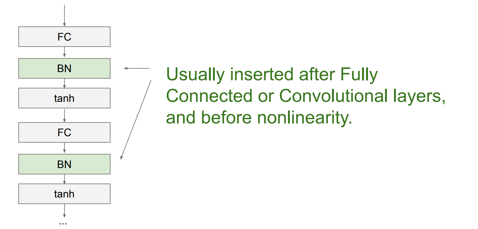
Batch Normalization
Force the inputs to be "nicely scaled" at each layer.
\(N\) : batch size
\(D\) : feature size
\(x\) : input with shape \(N\times D\)
\(\gamma\) : learnable scale and shift parameter with shape \(D\)
\(\beta\) : learnable scale and shift parameter with shape \(D\)
The procedure of batch normalization:
- Calculate channel-wise mean \(\mu_j=\frac{1}{N}\sum_{i=1}^Nx_{i,j}\\\) . The result \(\mu\) with shape \(D\) .
- Calculate channel-wise variance \(\sigma_j^2=\frac{1}{N}\sum_{i=1}^N(x_{i,j}-\mu_j)^2\\\) . The result \(\sigma^2\) with shape \(D\) .
- Calculate normalized \(\hat{x}_{i,j}=\frac{x_{i,j}-\mu_j}{\sqrt{\sigma_j^2+\epsilon}}\\\) . The result \(\hat{x}\) with shape \(N\times D\) .
- Scale normalized input to get output \(y_{i,j}=\gamma_j\hat{x}_{i,j}+\beta_j\) . The result \(y\) with shape \(N\times D\) .
Why scale: The constraint "zero-mean, unit variance" may be too hard.
Pros:
- Makes deep networks much easier to train!
- Improves gradient flow.
- Allows higher learning rates, faster convergence.
- Networks become more robust to initialization.
- Acts as regularization during training.
- Zero overhead at test-time: can be fused with conv!
Cons:
Behaves differently during training and testing: this is a very common source of bugs!
Transfer Learning
Train on a pre-trained model with other datasets.
An empirical suggestion:
| very similar dataset | very different dataset | |
|---|---|---|
| very little data | Use Linear Classifier on top layer. | You’re in trouble… Try linear classifier from different stages. |
| quite a lot of data | Finetune a few layers. | Finetune a larger number of layers. |
Regularization
Common Pattern of Regularization
Training: Add some kind of randomness. \(y=f(x,z)\)
Testing: Average out randomness (sometimes approximate). \(y=f(x)=E_z\big[f(x,z)\big]=\int p(z)f(x,z)dz\\\)
Regularization Term
L2 regularization: \(R(W)=\sum_k\sum_lW_{k,l}^2\) (weight decay)
L1 regularization: \(R(W)=\sum_k\sum_l|W_{k,l}|\)
Elastic net : \(R(W)=\sum_k\sum_l\big(\beta W_{k,l}^2+|W_{k,l}|\big)\) (L1+L2)
Dropout
Training: Randomly set some neurons to 0 with a probability \(p\) .
Testing: Each neuron multiplies by dropout probability \(p\) . (scale the output back)
More common: Scale the output with \(\frac{1}{p}\) when training, keep the original output when testing.
Why dropout works:
- Forces the network to have a redundant representation. Prevents co-adaptation of features.
- Another interpretation: Dropout is training a large ensemble of models (that share parameters).
Batch Normalization
See above.
Data Augmentation
- Horizontal Flips
- Random Crops and Scales
- Color Jitter
- Rotation
- Stretching
- Shearing
- Lens Distortions
- ...
There also exists automatic data augmentation method using neural networks.
Other Methods and Summary
DropConnect: Drop connections between neurons.
Fractional Max Pooling: Use randomized pooling regions.
Stochastic Depth: Skip some layers in the network.
Cutout: Set random image regions to zero.
Mixup: Train on random blends of images.
| Regularization Method | Usage |
|---|---|
| Dropout | For large fully-connected layers. |
| Batch Normalization & Data Augmentation | Almost always a good idea. |
| Cutout & Mixup | For small classification datasets. |
Hyperparameter Tuning
| Most Common Hyperparameters | Less Sensitive Hyperparameters |
|---|---|
| learning rate learning rate decay schedule weight decay | setting of momentum ... |
Tips on hyperparameter tuning:
- Prefer one validation fold to cross-validation.
- Search for hyperparameters on log scale. (e.g. multiply the hyperparameter by a fixed number \(k\) at each search)
- Prefer random search to grid search.
- Careful with best values on border.
- Stage your search from coarse to fine.
Implementation
Have a worker that continuously samples random hyperparameters and performs the optimization. During the training, the worker will keep track of the validation performance after every epoch, and writes a model checkpoint to a file.
Have a master that launches or kills workers across a computing cluster, and may additionally inspect the checkpoints written by workers and plot their training statistics.
Common Procedures
- Check initial loss.
Turn off weight decay, sanity check loss at initialization \(\log(C)\) for softmax with \(C\) classes.
- Overfit a small sample. (important)
Try to train to 100% training accuracy on a small sample of training data.
Fiddle with architecture, learning rate, weight initialization.
- Find learning rate that makes loss go down.
Use the architecture from the previous step, use all training data, turn on small weight decay, find a learning rate that makes the loss drop significantly within 100 iterations.
Good learning rates to try: \(0.1,0.01,0.001,0.0001,\dots\)
- Coarse grid, train for 1-5 epochs.
Choose a few values of learning rate and weight decay around what worked from Step 3, train a few models for 1-5 epochs.\
Good weight decay to try: \(0.0001,0.00001,0\)
- Refine grid, train longer.
Pick best models from Step 4, train them for longer (10-20 epochs) without learning rate decay.
- Look at loss and accuracy curves.
- GOTO step 5.
Gradient Checks
CS231n Convolutional Neural Networks for Visual Recognition
Compute analytical gradient manually using \(f_a'=\frac{\partial f(x)}{\partial x}=\frac{f(x-h)-f(x+h)}{2h}\\\)
Get relative error between numerical gradient \(f_n'\) and analytical gradient \(f_a'\) using \(E=\frac{|f_n'-f_a'|}{\max{|f_n'|,|f_a'|}}\\\)
| Relative Error | Result |
|---|---|
| \(E>10^{-2}\) | Probably \(f_n'\) is wrong. |
| \(10^{-2}>E>10^{-4}\) | Not good, should check the gradient. |
| \(10^{-4}>E>10^{-6}\) | Okay for objectives with kinks. (e.g. ReLU) Not good for objectives with no kink. (e.g. softmax, tanh) |
| \(10^{-7}>E\) | Good. |
Tips on gradient checks:
- Use double precision.
- Use only few data points.
- Careful about kinks in the objective. (e.g. \(x=0\) for ReLU activation)
- Careful with the step size \(h\).
- Use gradient check after the loss starts to go down.
- Remember to turn off anything that may affect the gradient. (e.g. regularization / dropout / augmentations)
- Check only few dimensions for every parameter. (reduce time cost)
8 - Visualizing and Understanding
Feature Visualization and Inversion
Visualizing what models have learned
| Visualize Areas | |
|---|---|
| Filters | Visualize the raw weights of each convolution kernel. (better in the first layer) |
| Final Layer Features | Run dimensionality reduction for features in the last FC layer. (PCA, t-SNE...) |
| Activations | Visualize activated areas. (Understanding Neural Networks Through Deep Visualization) |
Understanding input pixels
Maximally Activating Patches
- Pick a layer and a channel.
- Run many images through the network, record values of the chosen channel.
- Visualize image patches that correspond to maximal activation features.
For example, we have a layer with shape \(128\times13\times13\). We pick the 17th channel from all 128 channels. Then we run many pictures through the network. During each run we can find a maximal activation feature among all the \(13\times13\) features in channel 17. We then record the corresponding picture patch for each maximal activation feature. At last, we visualize all picture patches for each feature.
This will help us find the relationship between each maximal activation feature and its corresponding picture patches.
(each row of the following picture represents a feature)
Saliency via Occlusion
Mask part of the image before feeding to CNN, check how much predicted probabilities change.
Saliency via Backprop
- Compute gradient of (unnormalized) class score with respect to image pixels.
- Take absolute value and max over RGB channels to get saliency maps.
Intermediate Features via Guided Backprop
- Pick a single intermediate neuron. (e.g. one feature in a \(128\times13\times13\) feature map)
- Compute gradient of neuron value with respect to image pixels.
Striving for Simplicity: The All Convolutional Net
Just like "Maximally Activating Patches", this could find the part of an image that a neuron responds to.
Gradient Ascent
Generate a synthetic image that maximally activates a neuron.
- Initialize image \(I\) to zeros.
- Forward image to compute current scores \(S_c(I)\) (for class \(c\) before softmax).
- Backprop to get gradient of neuron value with respect to image pixels.
- Make a small update to the image.
Objective: \(\max S_c(I)-\lambda\lVert I\lVert^2\)
Deep Inside Convolutional Networks: Visualising Image Classification Models and Saliency Maps
Adversarial Examples
Find an fooling image that can make the network misclassify correctly-classified images when it is added to the image.
- Start from an arbitrary image.
- Pick an arbitrary class.
- Modify the image to maximize the class.
- Repeat until network is fooled.
DeepDream and Style Transfer
Feature Inversion
Given a CNN feature vector \(\Phi_0\) for an image, find a new image \(x\) that:
- Features of new image \(\Phi(x)\) matches the given feature vector \(\Phi_0\).
- "looks natural”. (image prior regularization)
Objective: \(\min \lVert\Phi(x)-\Phi_0\lVert+\lambda R(x)\)
Understanding Deep Image Representations by Inverting Them
DeepDream: Amplify Existing Features
Given an image, amplify the neuron activations at a layer to generate a new one.
- Forward: compute activations at chosen layer.
- Set gradient of chosen layer equal to its activation.
- Backward: Compute gradient on image.
- Update image.
Texture Synthesis
Nearest Neighbor
- Generate pixels one at a time in scanline order
- Form neighborhood of already generated pixels, copy the nearest neighbor from input.
Neural Texture Synthesis
Gram Matrix: 格拉姆矩阵(Gram matrix)详细解读
- Pretrain a CNN on ImageNet.
- Run input texture forward through CNN, record activations on every layer.
Layer \(i\) gives feature map of shape \(C_i\times H_i\times W_i\).
- At each layer compute the Gram matrix \(G_i\) giving outer product of features.
- Reshape feature map at layer \(i\) to \(C_i\times H_iW_i\).
- Compute the Gram matrix \(G_i\) with shape \(C_i\times C_i\).
- Initialize generated image from random noise.
- Pass generated image through CNN, compute Gram matrix \(\hat{G}_l\) on each layer.
- Compute loss: Weighted sum of L2 distance between Gram matrices.
- \(E_l=\frac{1}{aN_l^2M_l^2}\sum_{i,j}\Big(G_i^{(i,j)}-\hat{G}_i^{(i,j)}\Big)^2\\\)
- \(\mathcal{L}(\vec{x},\hat{\vec{x}})=\sum_{l=0}^L\omega_lE_l\\\)
- Backprop to get gradient on image.
- Make gradient step on image.
- GOTO 5.
Texture Synthesis Using Convolutional Neural Networks
Style Transfer
Feature + Gram Reconstruction
Problem: Style transfer requires many forward / backward passes. Very slow!
Fast Style Transfer
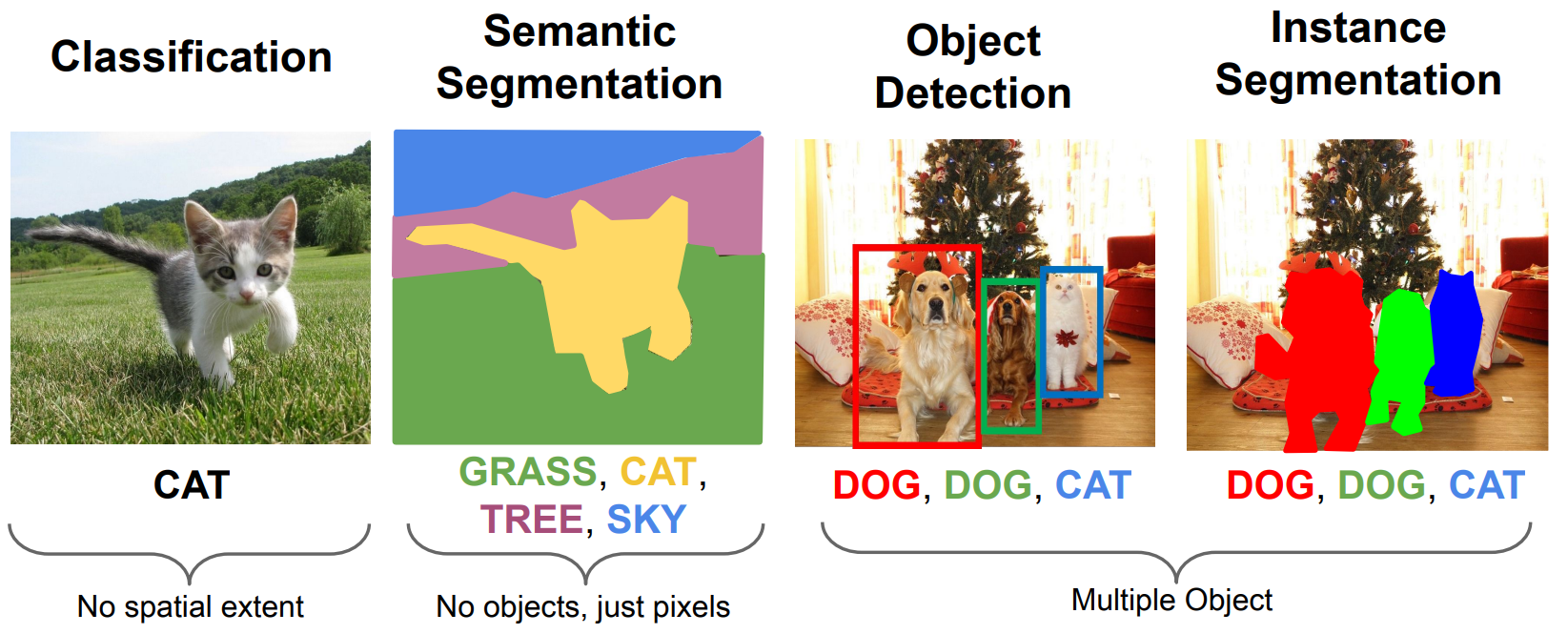
9 - Object Detection and Image Segmentation
Semantic Segmentation
Paired Training Data: For each training image, each pixel is labeled with a semantic category.
Fully Convolutional Network: Design a network with only convolutional layers without downsampling operators to make predictions for pixels all at once!
Problem: Convolutions at original image resolution will be very expensive...
Solution: Design fully convolutional network with downsampling and upsampling inside it!
- Downsampling: Pooling, strided convolution.
- Upsampling: Unpooling, transposed convolution.
Unpooling:
| Nearest Neighbor | "Bed of Nails" | "Position Memory" |
|---|---|---|
 |  |  |
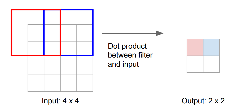
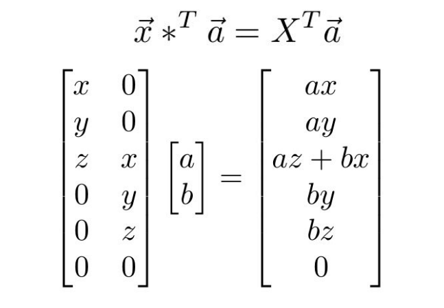
Transposed Convolution: (example size \(3\times3\), stride \(2\), pad \(1\))
| Normal Convolution | Transposed Convolution |
|---|---|
 |  |
 |  |
Object Detection
Single Object
Classification + Localization. (classification + regression problem)
Multiple Object
R-CNN
Using selective search to find “blobby” image regions that are likely to contain objects.
- Find regions of interest (RoI) using selective search. (region proposal)
- Forward each region through ConvNet.
- Classify features with SVMs.
Problem: Very slow. Need to do 2000 independent forward passes for each image!
Fast R-CNN
Pass the image through ConvNet before cropping. Crop the conv feature instead.
- Run whole image through ConvNet.
- Find regions of interest (RoI) from conv features using selective search. (region proposal)
- Classify RoIs using CNN.
Problem: Runtime is dominated by region proposals. (about \(90\%\) time cost)
Faster R-CNN
Insert Region Proposal Network (RPN) to predict proposals from features.
Otherwise same as Fast R-CNN: Crop features for each proposal, classify each one.
Region Proposal Network (RPN) : Slide many fixed windows over ConvNet features.
- Treat each point in the feature map as the anchor.
We have \(k\) fixed windows (anchor boxes) of different size/scale centered with each anchor.
- For each anchor box, predict whether it contains an object.
For positive boxes, also predict a corrections to the ground-truth box.
- Slide anchor over the feature map, get the “objectness” score for each box at each point.
- Sort the “objectness” score, take top \(300\) as the proposals.
Faster R-CNN is a Two-stage object detector:
- First stage: Run once per image
Backbone network
Region proposal network
- Second stage: Run once per region
Crop features: RoI pool / align
Predict object class
Prediction bbox offset
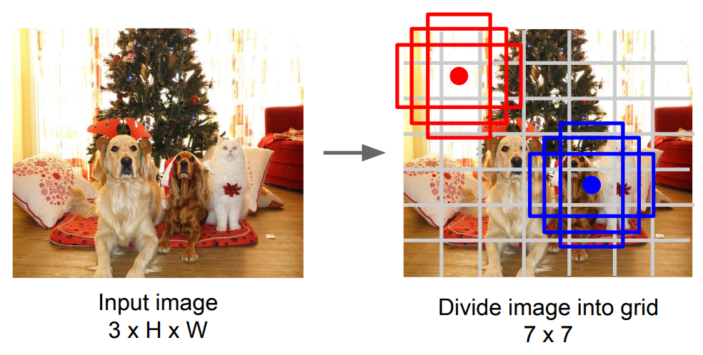
Single-Stage Object Detectors: YOLO
You Only Look Once: Unified, Real-Time Object Detection
- Divide image into grids. (example image grids shape \(7\times7\))
- Set anchors in the middle of each grid.
- For each grid: - Using \(B\) anchor boxes to regress \(5\) numbers: \(\text{dx, dy, dh, dw, confidence}\). - Predict scores for each of \(C\) classes.
- Finally the output is \(7\times7\times(5B+C)\).
Instance Segmentation
Mask R-CNN: Add a small mask network that operates on each RoI and predicts a \(28\times28\) binary mask.
Mask R-CNN performs very good results!
10 - Recurrent Neural Networks
Supplement content added according to Deep Learning Book - RNN.
Recurrent Neural Network (RNN)
Motivation: Sequence Processing
| One to One | One to Many | Many to One | Many to Many | Many to Many |
|---|---|---|---|---|
 |  |  |  |  |
| Vanilla Neural Networks | Image Captioning | Action Prediction | Video Captioning | Video Classification on Frame Level |
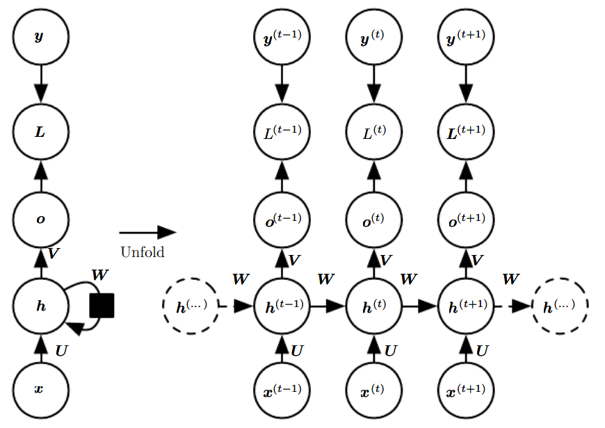
Vanilla RNN
\(x^{(t)}\) : Input at time \(t\).
\(h^{(t)}\) : State at time \(t\).
\(o^{(t)}\) : Output at time \(t\).
\(y^{(t)}\) : Expected output at time \(t\).
Many to One
| Calculation | |
|---|---|
| State Transition | \(h^{(t)}=\tanh(Wh^{(t-1)}+Ux^{(t)}+b)\) |
| Output Calculation | \(o^{(\tau)}=\text{sigmoid}\ \big(Vh^{(\tau)}+c\big)\) |
Many to Many (type 2)
| Calculation | |
|---|---|
| State Transition | \(h^{(t)}=\tanh(Wh^{(t-1)}+Ux^{(t)}+b)\) |
| Output Calculation | \(o^{(t)}=\text{sigmoid}\ \big(Vh^{(t)}+c\big)\) |
RNN with Teacher Forcing
Update current state according to last-time output instead of last-time state.
| Calculation | |
|---|---|
| State Transition | \(h^{(t)}=\tanh(Wo^{(t-1)}+Ux^{(t)}+b)\) |
| Output Calculation | \(o^{(t)}=\text{sigmoid}\ \big(Vh^{(t)}+c\big)\) |
RNN with "Output Forwarding"
We can also combine last-state output with this-state input together.
| Calculation | |
|---|---|
| State Transition (training) | \(h^{(t)}=\tanh(Wh^{(t-1)}+Ux^{(t)}+Ry^{(t-1)}+b)\) |
| State Transition (testing) | \(h^{(t)}=\tanh(Wh^{(t-1)}+Ux^{(t)}+Ro^{(t-1)}+b)\) |
| Output Calculation | \(o^{(t)}=\text{sigmoid}\ \big(Vh^{(t)}+c\big)\) |
Usually we use \(o^{(t-1)}\) in place of \(y^{(t-1)}\) at testing time.
Bidirectional RNN
When dealing with a whole input sequence, we can process features from two directions.
| Calculation | |
|---|---|
| State Transition (forward) | \(h^{(t)}=\tanh(W_1h^{(t-1)}+U_1x^{(t)}+b_1)\) |
| State Transition (backward) | \(g^{(t)}=\tanh(W_2g^{(t+1)}+U_2x^{(t)}+b_2)\) |
| Output Calculation | \(o^{(t)}=\text{sigmoid}\ \big(Vh^{(t)}+Wg^{(t)}+c\big)\) |
Encoder-Decoder Sequence to Sequence RNN
This is a many-to-many structure (type 1).
First we encode information according to \(x\) with no output.
Later we decode information according to \(y\) with no input.
\(C\) : Context vector, often \(C=h^{(T)}\) (last state of encoder).
| Calculation | |
|---|---|
| State Transition (encode) | \(h^{(t)}=\tanh(W_1h^{(t-1)}+U_1x^{(t)}+b_1)\) |
| State Transition (decode, training) | \(s^{(t)}=\tanh(W_2s^{(t-1)}+U_2y^{(t)}+TC+b_2)\) |
| State Transition (decode, testing) | \(s^{(t)}=\tanh(W_2s^{(t-1)}+U_2o^{(t)}+TC+b_2)\) |
| Output Calculation | \(o^{(t)}=\text{sigmoid}\ \big(Vs^{(t)}+c\big)\) |
Example: Image Captioning
Summary
Advantages of RNN:
- Can process any length input.
- Computation for step \(t\) can (in theory) use information from many steps back.
- Model size doesn’t increase for longer input.
- Same weights applied on every timestep, so there is symmetry in how inputs are processed.
Disadvantages of RNN:
- Recurrent computation is slow.
- In practice, difficult to access information from many steps back.
- Problems with gradient exploding and gradient vanishing. (check Deep Learning Book - RNN Page 396, Chap 10.7)
Long Short Term Memory (LSTM)
Add a "cell block" to store history weights.
\(c^{(t)}\) : Cell at time \(t\).
\(f^{(t)}\) : Forget gate at time \(t\). Deciding whether to erase the cell.
\(i^{(t)}\) : Input gate at time \(t\). Deciding whether to write to the cell.
\(g^{(t)}\) : External input gate at time \(t\). Deciding how much to write to the cell.
\(o^{(t)}\) : Output gate at time \(t\). Deciding how much to reveal the cell.
| Calculation (Gate) | |
|---|---|
| Forget Gate | \(f^{(t)}=\text{sigmoid}\ \big(W_fh^{(t-1)}+U_fx^{(t)}+b_f\big)\) |
| Input Gate | \(i^{(t)}=\text{sigmoid}\ \big(W_ih^{(t-1)}+U_ix^{(t)}+b_i\big)\) |
| External Input Gate | \(g^{(t)}=\tanh(W_gh^{(t-1)}+U_gx^{(t)}+b_g)\) |
| Output Gate | \(o^{(t)}=\text{sigmoid}\ \big(W_oh^{(t-1)}+U_ox^{(t)}+b_o\big)\) |
| Calculation (Main) | |
|---|---|
| Cell Transition | \(c^{(t)}=f^{(t)}\odot c^{(t-1)}+i^{(t)}\odot g^{(t)}\) |
| State Transition | \(h^{(t)}=o^{(t)}\odot\tanh(c^{(t)})\) |
| Output Calculation | \(O^{(t)}=\text{sigmoid}\ \big(Vh^{(t)}+c\big)\) |
Other RNN Variants
GRU...
11 - Attention and Transformers
RNN with Attention
Encoder-Decoder Sequence to Sequence RNN Problem:
Input sequence bottlenecked through a fixed-sized context vector \(C\). (e.g. \(T=1000\))
Intuitive Solution:
Generate new context vector \(C_t\) at each step \(t\) !
\(e_{t,i}\) : Alignment score for input \(i\) at state \(t\). (scalar)
\(a_{t,i}\) : Attention weight for input \(i\) at state \(t\).
\(C_t\) : Context vector at state \(t\).
| Calculation | |
|---|---|
| Alignment Score | \(e_i^{(t)}=f(s^{(t-1)},h^{(i)})\). Where \(f\) is an MLP. |
| Attention Weight | \(a_i^{(t)}=\text{softmax}\ (e_i^{(t)})\). Softmax includes all \(e_i\) at state \(t\). |
| Context Vector | \(C^{(t)}=\sum_i a_i^{(t)}h^{(i)}\) |
| Decoder State Transition | \(s^{(t)}=\tanh(Ws^{(t-1)}+Uy^{(t)}+TC^{(t)}+b)\) |
Example on Image Captioning:
General Attention Layer
Add linear transformations to the input vector before attention.
Notice:
- Number of queries \(q\) is variant. (can be different from the number of keys \(k\))
- Number of outputs \(y\) is equal to the number of queries \(q\).
Each \(y\) is a linear weighting of values \(v\).
- Alignment \(e\) is divided by \(\sqrt{D}\) to avoid "explosion of softmax", where \(D\) is the dimension of input feature.
Self-attention Layer
The query vectors \(q\) are also generated from the inputs.
In this way, the shape of \(y\) is equal to the shape of \(x\).
Example with CNN:
Positional Encoding
Self-attention layer doesn’t care about the orders of the inputs!
To encode ordered sequences like language or spatially ordered image features, we can add positional encoding to the inputs.
We use a function \(P:R\rightarrow R^d\) to process the position \(i\) into a d-dimensional vector \(p_i=P(i)\).
| Constraint Condition of \(P\) | |
|---|---|
| Uniqueness | \(P(i)\ne P(j)\) |
| Equidistance | \(\lVert P(i+k)-P(i)\rVert^2=\lVert P(j+k)-P(j)\rVert^2\) |
| Boundness | \(P(i)\in[a,b]\) |
| Determinacy | \(P(i)\) is always a static value. (function is not dynamic) |
We can either train a encoder model, or design a fixed function.
A Practical Positional Encoding Method: Using \(\sin\) and \(\cos\) with different frequency \(\omega\) at different dimension.
\(P(t)=\begin{bmatrix}\sin(\omega_1,t)\\\cos(\omega_1,t)\\\\\sin(\omega_2,t)\\\cos(\omega_2,t)\\\vdots\\\sin(\omega_{\frac{d}{2}},t)\\\cos(\omega_{\frac{d}{2}},t)\end{bmatrix}\), where frequency \(\omega_k=\frac{1}{10000^{\frac{2k}{d}}}\\\). (wave length \(\lambda=\frac{1}{\omega}=10000^{\frac{2k}{d}}\\\))
\(P(t)=\begin{bmatrix}\sin(1/10000^{\frac{2}{d}},t)\\\cos(1/10000^{\frac{2}{d}},t)\\\\\sin(1/10000^{\frac{4}{d}},t)\\\cos(1/10000^{\frac{4}{d}},t)\\\vdots\\\sin(1/10000^1,t)\\\cos(1/10000^1,t)\end{bmatrix}\), after we substitute \(\omega_k\) into the equation.
\(P(t)\) is a vector with size \(d\), where \(d\) is a hyperparameter to choose according to the length of input sequence.
An intuition of this method is the binary encoding of numbers.
[lecture 11d] 注意力和 transformer (positional encoding 补充,代码实现,距离计算 )
It is easy to prove that \(P(t)\) satisfies "Equidistance": (set \(d=2\) for example)
\(\begin{aligned}\lVert P(i+k)-P(i)\rVert^2&=\big[\sin(\omega_1,i+k)-\sin(\omega_1,i)\big]^2+\big[\cos(\omega_1,i+k)-\cos(\omega_1,i)\big]^2\\&=2-2\sin(\omega_1,i+k)\sin(\omega_1,i)-2\cos(\omega_1,i+k)\cos(\omega_1,i)\\&=2-2\cos(\omega_1,k)\end{aligned}\)
So the distance is not associated with \(i\), we have \(\lVert P(i+k)-P(i)\rVert^2=\lVert P(j+k)-P(j)\rVert^2\).
Visualization of \(P(t)\) features: (set \(d=32\), \(x\) axis represents the position of sequence)
Masked Self-attention Layer
To prevent vectors from looking at future vectors, we manually set alignment scores to \(-\infty\).
Multi-head Self-attention Layer
Multiple self-attention heads in parallel.
Transformer
Encoder Block
Inputs: Set of vectors \(z\). (in which \(z_i\) can be a word in a sentence, or a pixel in a picture...)
Output: Set of context vectors \(c\). (encoded features of \(z\))
The number of blocks \(N=6\) in original paper.
Notice:
- Self-attention is the only interaction between vectors \(x_0,x_1,\dots,x_n\).
- Layer norm and MLP operate independently per vector.
- Highly scalable, highly parallelizable, but high memory usage.
Decoder Block
Inputs: Set of vectors \(y\). (\(y_i\) can be a word in a sentence, or a pixel in a picture...)
Inputs: Set of context vectors \(c\).
Output: Set of vectors \(y'\). (decoded result, \(y'_i=y_{i+1}\) for the first \(n-1\) number of \(y'\))
The number of blocks \(N=6\) in original paper.
Notice:
- Masked self-attention only interacts with past inputs.
- Multi-head attention block is NOT self-attention. It attends over encoder outputs.
- Highly scalable, highly parallelizable, but high memory usage. (same as encoder)
Why we need mask in decoder:
- Needs for the special formation of output \(y'_i=y_{i+1}\).
- Needs for parallel computation.
在测试或者预测时,Transformer 里 decoder 为什么还需要 seq mask?
Example on Image Captioning (Only with Transformers)
Comparing RNNs to Transformer
| RNNs | Transformer | |
|---|---|---|
| Pros | LSTMs work reasonably well for long sequences. | 1. Good at long sequences. Each attention calculation looks at all inputs. 2. Can operate over unordered sets or ordered sequences with positional encodings. 3. Parallel computation: All alignment and attention scores for all inputs can be done in parallel. |
| Cons | 1. Expects an ordered sequences of inputs. 2. Sequential computation: Subsequent hidden states can only be computed after the previous ones are done. | Requires a lot of memory: \(N\times M\) alignment and attention scalers need to be calculated and stored for a single self-attention head. |
Comparing ConvNets to Transformer
ConvNets strike back!
12 - Video Understanding
Video Classification
Take video classification task for example.
Input size: \(C\times T\times H\times W\).
The problem is, videos are quite big. We can't afford to train on raw videos, instead we train on video clips.
| Raw Videos | Video Clips |
|---|---|
| \(1920\times1080,\ 30\text{fps}\) | \(112\times112,\ 5\text{f}/3.2\text{s}\) |
| \(10\text{GB}/\text{min}\) | \(588\text{KB}/\text{min}\) |
Plain CNN Structure
Single Frame 2D-CNN
Train a normal 2D-CNN model.
Classify each frame independently.
Average the result of each frame as the final result.
Late Fusion
Get high-level appearance of each frame, and combine them.
Run 2D-CNN on each frame, pool features and feed to Linear Layers.
Problem: Hard to compare low-level motion between frames.
Early Fusion
Compare frames with very first Conv Layer, after that normal 2D-CNN.
Problem: One layer of temporal processing may not be enough!
3D-CNN
Convolve on 3 dimensions: Height, Width, Time.
Input size: \(C_{in}\times T\times H\times W\).
Kernel size: \(C_{in}\times C_{out}\times 3\times 3\times 3\).
Output size: \(C_{out}\times T\times H\times W\). (with zero paddling)
C3D (VGG of 3D-CNNs)
The cost is quite expensive...
| Network | Calculation |
|---|---|
| AlexNet | 0.7 GFLOP |
| VGG-16 | 13.6 GFLOP |
| C3D | 39.5 GFLOP |
Two-Stream Networks
Separate motion and appearance.
I3D (Inflating 2D Networks to 3D)
Take a 2D-CNN architecture.
Replace each 2D conv/pool layer with a 3D version.
Modeling Long-term Temporal Structure
Recurrent Convolutional Network
Similar to multi-layer RNN, we replace the dot-product operation with convolution.
Feature size in layer \(L\), time \(t-1\): \(W_h\times H\times W\).
Feature size in layer \(L-1\), time \(t\): \(W_x\times H\times W\).
Feature size in layer \(L\), time \(t\): \((W_h+W_x)\times H\times W\).
Problem: RNNs are slow for long sequences. (can’t be parallelized)
Spatio-temporal Self-attention
Introduce self-attention into video classification problems.
Vision Transformers for Video
Factorized attention: Attend over space / time.
So many papers...
Visualizing Video Models
Multimodal Video Understanding
Temporal Action Localization
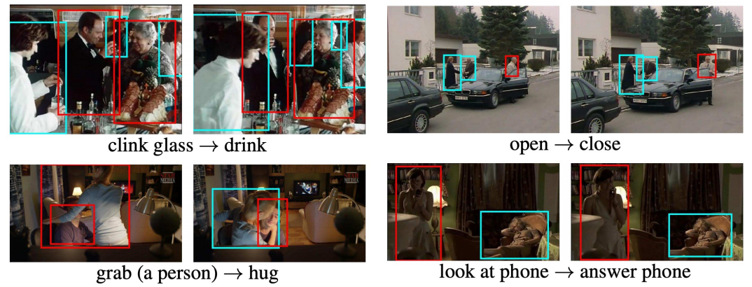
Given a long untrimmed video sequence, identify frames corresponding to different actions.
Spatio-Temporal Detection
Given a long untrimmed video, detect all the people in both space and time and classify the activities they are performing.
Visually-guided Audio Source Separation
And So on...
13 - Generative Models
PixelRNN and PixelCNN
Fully Visible Belief Network (FVBN)
\(p(x)\) : Likelihood of image \(x\).
\(p(x_1,x_2,\dots,x_n)\) : Joint likelihood of all \(n\) pixels in image \(x\).
\(p(x_i|x_1,x_2,\dots,x_{i-1})\) : Probability of pixel \(i\) value given all previous pixels.
For explicit density models, we have \(p(x)=p(x_1,x_2,\dots,x_n)=\prod_{i=1}^np(x_i|x_1,x_2,\dots,x_{i-1})\\\).
Objective: Maximize the likelihood of training data.
PixelRNN
Generate image pixels starting from corner.
Dependency on previous pixels modeled using an RNN (LSTM).
Drawback: Sequential generation is slow in both training and inference!
PixelCNN
Still generate image pixels starting from corner.
Dependency on previous pixels modeled using a CNN over context region (masked convolution).
Drawback: Though its training is faster, its generation is still slow. (pixel by pixel)
Variational Autoencoder
Supplement content added according to Tutorial on Variational Autoencoders. (paper with notes: VAE Tutorial.pdf)
Autoencoder
Learn a lower-dimensional feature representation with unsupervised approaches.
\(x\rightarrow z\) : Dimension reduction for input features.
\(z\rightarrow \hat{x}\) : Reconstruct input features.
After training, we throw the decoder away and use the encoder for transferring.
For generative models, there is a problem:
We can’t generate new images from an autoencoder because we don’t know the space of \(z\).
Variational Autoencoder
Character Description
\(X\) : Images. (random variable)
\(Z\) : Latent representations. (random variable)
\(P(X)\) : True distribution of all training images \(X\).
\(P(Z)\) : True distribution of all latent representations \(Z\).
\(P(X|Z)\) : True posterior distribution of all images \(X\) with condition \(Z\).
\(P(Z|X)\) : True prior distribution of all latent representations \(Z\) with condition \(X\).
\(Q(Z|X)\) : Approximated prior distribution of all latent representations \(Z\) with condition \(X\).
\(x\) : A specific image.
\(z\) : A specific latent representation.
\(\theta\): Learned parameters in decoder network.
\(\phi\): Learned parameters in encoder network.
\(p_\theta(x)\) : Probability that \(x\sim P(X)\).
\(p_\theta(z)\) : Probability that \(z\sim P(Z)\).
\(p_\theta(x|z)\) : Probability that \(x\sim P(X|Z)\).
\(p_\theta(z|x)\) : Probability that \(z\sim P(Z|X)\).
\(q_\phi(z|x)\) : Probability that \(z\sim Q(Z|X)\).
Decoder
Objective:
Generate new images from \(\mathscr{z}\).
- Generate a value \(z^{(i)}\) from the prior distribution \(P(Z)\).
- Generate a value \(x^{(i)}\) from the conditional distribution \(P(X|Z)\).
Lemma:
Any distribution in \(d\) dimensions can be generated by taking a set of \(d\) variables that are normally distributed and mapping them through a sufficiently complicated function. (source: Tutorial on Variational Autoencoders, Page 6)
Solutions:
- Choose prior distribution \(P(Z)\) to be a simple distribution, for example \(P(Z)\sim N(0,1)\).
- Learn the conditional distribution \(P(X|Z)\) through a neural network (decoder) with parameter \(\theta\).
Encoder
Objective:
Learn \(\mathscr{z}\) with training images.
Given: (From the decoder, we can deduce the following probabilities.)
- data likelihood: \(p_\theta(x)=\int p_\theta(x|z)p_\theta(z)dz\).
- posterior density: \(p_\theta(z|x)=\frac{p_\theta(x|z)p_\theta(z)}{p_\theta(x)}=\frac{p_\theta(x|z)p_\theta(z)}{\int p_\theta(x|z)p_\theta(z)dz}\).
Problem:
Both \(p_\theta(x)\) and \(p_\theta(z|x)\) are intractable. (can't be optimized directly as they contain integral operation)
Solution:
Learn \(Q(Z|X)\) to approximate the true posterior \(P(Z|X)\).
Use \(q_\phi(z|x)\) in place of \(p_\theta(z|x)\).
Variational Autoencoder (Combination of Encoder and Decoder)
Objective:
Maximize \(p_\theta(x)\) for all \(x^{(i)}\) in the training set.
$$ \begin{aligned} \log p_\theta\big(x^{(i)}\big)&=\mathbb{E}{z\sim q\phi\big(z|x^{(i)}\big)}\Big[\log p_\theta\big(x^{(i)}\big)\Big]\
&=\mathbb{E}z\Bigg[\log\frac{p\theta\big(x^{(i)}|z\big)p_\theta\big(z\big)}{p_\theta\big(z|x^{(i)}\big)}\Bigg]\quad\text{(Bayes' Rule)}\
&=\mathbb{E}z\Bigg[\log\frac{p\theta\big(x^{(i)}|z\big)p_\theta\big(z\big)}{p_\theta\big(z|x^{(i)}\big)}\frac{q_\phi\big(z|x^{(i)}\big)}{q_\phi\big(z|x^{(i)}\big)}\Bigg]\quad\text{(Multiply by Constant)}\
&=\mathbb{E}z\Big[\log p\theta\big(x^{(i)}|z\big)\Big]-\mathbb{E}z\Bigg[\log\frac{q\phi\big(z|x^{(i)}\big)}{p_\theta\big(z\big)}\Bigg]+\mathbb{E}z\Bigg[\log\frac{p\theta\big(z|x^{(i)}\big)}{q_\phi\big(z|x^{(i)}\big)}\Bigg]\quad\text{(Logarithm)}\
&=\mathbb{E}z\Big[\log p\theta\big(x^{(i)}|z\big)\Big]-D_{\text{KL}}\Big[q_\phi\big(z|x^{(i)}\big)||p_\theta\big(z\big)\Big]+D_{\text{KL}}\Big[p_\theta\big(z|x^{(i)}\big)||q_\phi\big(z|x^{(i)}\big)\Big]\quad\text{(KL Divergence)} \end{aligned} $$
Analyze the Formula by Term:
\(\mathbb{E}_z\Big[\log p_\theta\big(x^{(i)}|z\big)\Big]\): Decoder network gives \(p_\theta\big(x^{(i)}|z\big)\), can compute estimate of this term through sampling.
\(D_{\text{KL}}\Big[q_\phi\big(z|x^{(i)}\big)||p_\theta\big(z\big)\Big]\): This KL term (between Gaussians for encoder and \(z\) prior) has nice closed-form solution!
\(D_{\text{KL}}\Big[p_\theta\big(z|x^{(i)}\big)||q_\phi\big(z|x^{(i)}\big)\Big]\): The part \(p_\theta\big(z|x^{(i)}\big)\) is intractable. However, we know KL divergence always \(\ge0\).
Tractable Lower Bound:
We can maximize the lower bound of that formula.
As \(D_{\text{KL}}\Big[p_\theta\big(z|x^{(i)}\big)||q_\phi\big(z|x^{(i)}\big)\Big]\ge0\) , we can deduce that:
$$ \begin{aligned} \log p_\theta\big(x^{(i)}\big)&=\mathbb{E}z\Big[\log p\theta\big(x^{(i)}|z\big)\Big]-D_{\text{KL}}\Big[q_\phi\big(z|x^{(i)}\big)||p_\theta\big(z\big)\Big]+D_{\text{KL}}\Big[p_\theta\big(z|x^{(i)}\big)||q_\phi\big(z|x^{(i)}\big)\Big]\
&\ge\mathbb{E}z\Big[\log p\theta\big(x^{(i)}|z\big)\Big]-D_{\text{KL}}\Big[q_\phi\big(z|x^{(i)}\big)||p_\theta\big(z\big)\Big] \end{aligned} $$
So the loss function \(\mathcal{L}\big(x^{(i)},\theta,\phi\big)=-\mathbb{E}_z\Big[\log p_\theta\big(x^{(i)}|z\big)\Big]+D_{\text{KL}}\Big[q_\phi\big(z|x^{(i)}\big)||p_\theta\big(z\big)\Big]\).
\(\mathbb{E}_z\Big[\log p_\theta\big(x^{(i)}|z\big)\Big]\): Decoder, reconstruct the input data.
\(D_{\text{KL}}\Big[q_\phi\big(z|x^{(i)}\big)||p_\theta\big(z\big)\Big]\): Encoder, make approximate posterior distribution close to prior.
Generative Adversarial Networks (GANs)
Motivation & Modeling
Objective: Not modeling any explicit density function.
Problem: Want to sample from complex, high-dimensional training distribution. No direct way to do this!
Solution: Sample from a simple distribution, e.g. random noise. Learn the transformation to training distribution.
Problem: We can't learn the mapping relation between sample \(z\) and training images.
Solution: Use a discriminator network to tell whether the generate image is within data distribution or not.
Discriminator network: Try to distinguish between real and fake images.
Generator network: Try to fool the discriminator by generating real-looking images.
\(x\) : Real data.
\(y\) : Fake data, which is generated by the generator network. \(y=G_{\theta_g}(z)\).
\(D_{\theta_d}(x)\) : Discriminator score, which is the likelihood of real image. \(D_{\theta_d}(x)\in[0,1]\).
Objective of discriminator network:
\(\max_{\theta_d}\bigg[\mathbb{E}_x\Big(\log D_{\theta_d}(x)\Big)+\mathbb{E}_{z\sim p(z)}\Big(\log\big(1-D_{\theta_d}(y)\big)\Big)\bigg]\)
Objective of generator network:
\(\min_{\theta_g}\max_{\theta_d}\bigg[\mathbb{E}_x\Big(\log D_{\theta_d}(x)\Big)+\mathbb{E}_{z\sim p(z)}\Big(\log\big(1-D_{\theta_d}(y)\big)\Big)\bigg]\)
Training Strategy
Two combine this two networks together, we can train them alternately:
- Gradient ascent on discriminator.
\(\max_{\theta_d}\bigg[\mathbb{E}_x\Big(\log D_{\theta_d}(x)\Big)+\mathbb{E}_{z\sim p(z)}\Big(\log\big(1-D_{\theta_d}(y)\big)\Big)\bigg]\)
- Gradient descent on generator.
\(\min_{\theta_g}\bigg[\mathbb{E}_{z\sim p(z)}\Big(\log\big(1-D_{\theta_d}(y)\big)\Big)\bigg]\)
However, the gradient of generator decreases with the value itself, making it hard to optimize.
So we replace \(\log\big(1-D_{\theta_d}(y)\big)\) with \(-\log D_{\theta_d}(y)\), and use gradient ascent instead.
- Gradient ascent on discriminator.
\(\max_{\theta_d}\bigg[\mathbb{E}_x\Big(\log D_{\theta_d}(x)\Big)+\mathbb{E}_{z\sim p(z)}\Big(\log\big(1-D_{\theta_d}(y)\big)\Big)\bigg]\)
- Gradient ascent on generator.
\(\max_{\theta_g}\bigg[\mathbb{E}_{z\sim p(z)}\Big(\log D_{\theta_d}(y)\Big)\bigg]\)
Summary
Pros: Beautiful, state-of-the-art samples!
Cons:
- Trickier / more unstable to train.
- Can’t solve inference queries such as \(p(x), p(z|x)\).
14 - Self-supervised Learning
Aim: Solve “pretext” tasks that produce good features for downstream tasks.
Application:
- Learn a feature extractor from pretext tasks. (self-supervised)
- Attach a shallow network on the feature extractor.
- Train the shallow network on target task with small amount of labeled data. (supervised)
Pretext Tasks
Labels are generated automatically.
Rotation
Train a classifier on randomly rotated images.
Rearrangement
Train a classifier on randomly shuffled image pieces.
Predict the location of image pieces.
Inpainting
Mask part of the image, train a network to predict the masked area.
Method referencing Context Encoders: Feature Learning by Inpainting.
Combine two types of loss together to get better performance:
- Reconstruction loss (L2 loss): Used for reconstructing global features.
- Adversarial loss: Used for generating texture features.
Coloring
Transfer between greyscale images and colored images.
Cross-channel predictions for images: Split-Brain Autoencoders.
Video coloring: Establish mappings between reference and target frames in a learned feature space. Tracking Emerges by Colorizing Videos.
Summary for Pretext Tasks
- Pretext tasks focus on “visual common sense”.
- The models are forced learn good features about natural images.
- We don’t care about the performance of these pretext tasks.
What we care is the performance of downstream tasks.
Problems of Specific Pretext Tasks
- Coming up with individual pretext tasks is tedious.
- The learned representations may not be general.
Intuitive Solution: Contrastive Learning.
Contrastive Representation Learning
Local additional references: Contrastive Learning.md.
Objective:
Given a chosen score function \(s\), we aim to learn an encoder function \(f\) that yields:
- For each sample \(x\), increase the similarity \(s\big(f(x),f(x^+)\big)\) between \(x\) and positive samples \(x^+\).
- Finally we want \(s\big(f(x),f(x^+)\big)\gg s\big(f(x),f(x^-)\big)\).
Loss Function:
Given \(1\) positive sample and \(N-1\) negative samples:
| InfoNCE Loss | Cross Entropy Loss |
|---|---|
| \(\begin{aligned}\mathcal{L}=-\mathbb{E}_X\Bigg[\log\frac{\exp{s\big(f(x),f(x^+)\big)}}{\exp{s\big(f(x),f(x^+)\big)}+\sum_{j=1}^{N-1}\exp{s\big(f(x),f(x^+)\big)}}\Bigg]\\\end{aligned}\) | \(\begin{aligned}\mathcal{L}&=-\sum_{i=1}^Np(x_i)\log q(x_i)\\&=-\mathbb{E}_X\big[\log q(x)\big]\\&=-\mathbb{E}_X\Bigg[\log\frac{\exp(x)}{\sum_{j=1}^N\exp(x_j)}\Bigg]\end{aligned}\) |
The InfoNCE Loss is a lower bound on the mutual information between \(f(x)\) and \(f(x^+)\):
\(\text{MI}\big[f(x),f(x^+)\big]\ge\log(N)-\mathcal{L}\)
The larger the negative sample size \(N\), the tighter the bound.
So we use \(N-1\) negative samples.
Instance Contrastive Learning
SimCLR
Use a projection function \(g(\cdot)\) to project features to a space where contrastive learning is applied.
The extra projection contributes a lot to the final performance.
Score Function: Cos similarity \(s(u,v)=\frac{u^Tv}{||u||||v||}\\\).
Positive Pair: Pair of augmented data.
Momentum Contrastive Learning (MoCo)
There are mainly \(3\) training strategy in contrastive learning:
- end-to-end: Keys are updated together with queries, e.g. SimCLR.
(limited by GPU size)
- memory bank: Store last-time keys for sampling.
(inconsistency between \(q\) and \(k\))
- MoCo: Use momentum methods to encode keys.
(combination of end-to-end & memory bank)
Key differences to SimCLR:
- Keep a running queue of keys (negative samples).
- Compute gradients and update the encoder only through the queries.
- Decouple min-batch size with the number of keys: can support a large number of negative samples.
- The key encoder is slowly progressing through the momentum update rules:
\(\theta_k\leftarrow m\theta_k+(1-m)\theta_q\)
Sequence Contrastive Learning
Contrastive Predictive Coding (CPC)
Contrastive: Contrast between “right” and “wrong” sequences using contrastive learning.
Predictive: The model has to predict future patterns given the current context.
Coding: The model learns useful feature vectors, or “code”, for downstream tasks, similar to other self-supervised methods.
Other Examples (Frontier)
Contrastive Language Image Pre-training (CLIP)
Contrastive learning between image and natural language sentences.
15 - Low-Level Vision
Pass...
16 - 3D Vision
Representation
Explicit vs Implicit
Explicit: Easy to sample examples, hard to do inside/outside check.
Implicit: Hard to sample examples, easy to do inside/outside check.
| Non-parametric | Parametric | |
|---|---|---|
| Explicit | Points. Meshes. | Splines. Subdivision Surfaces. |
| Implicit | Level Sets. Voxels. | Algebraic Surfaces. Constructive Solid Geometry. |
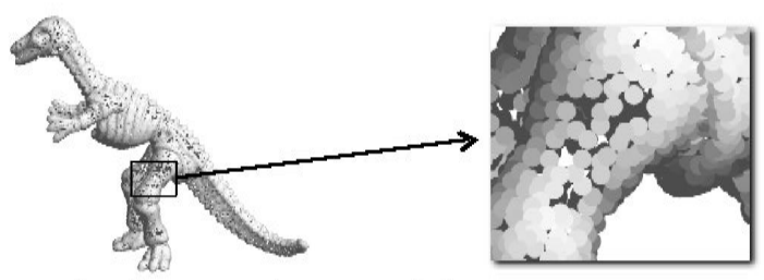
Point Clouds
The simplest representation.
Collection of \((x,y,z)\) coordinates.
Cons:
- Difficult to draw in under-sampled regions.
- No simplification or subdivision.
- No direction smooth rendering.
- No topological information.
Polygonal Meshes
Collection of vertices \(v\) and edges \(e\).
Pros:
- Can apply downsampling or upsampling on meshes.
- Error decreases by \(O(n^2)\) while meshes increase by \(O(n)\).
- Can approximate arbitrary topology.
- Efficient rendering.
Splines
Use specific functions to approximate the surface. (e.g. Bézier Curves)
Algebraic Surfaces
Use specific functions to represent the surface.
Constructive Solid Geometry
Combine implicit geometry with Boolean operations.
Level Sets
Store a grim of values to approximate the function.
Surface is found where interpolated value equals to \(0\).
Voxels
Binary thresholding the volumetric grid.
AI + 3D
Pass...


